Object fine-grained discrimination as a sensitive cognitive marker of transentorhinal integrity

Participants

A total of 51 participants took part in the study. Participants were community-dwelling, nominally healthy, older adults, between 65 and 83 years old, with no neurologic or psychiatric history, no MRI contraindication, and normal or corrected-to-normal vision. Participants’ high-level visual abilities were screened using the Overlapping Figures Task of the Birmingham Object Recognition Battery (BORB)⁷¹which did not lead to the exclusion of any participant. Cognitive status was assessed using the Montreal Cognitive Assessment (MoCA)⁷²but no participant was excluded on that basis, as we aimed for a participant group with a good distribution of cognitive abilities and MTL integrity, following previous studies⁵⁹ and as the presence of mild cognitive impairment detected through the MoCA is associated with tErC volume loss⁵². Every day, cognitive functioning was characterised using the ECog questionnaire⁷³. The study was approved by the Ethics Committee of the Liège University Hospital, and participants signed an informed consent before taking part to the experiment. Participants’ demographic information is presented in Table2.

Data from one participant was discarded in the odd-one-out task for objects, from four participants in the memory task for objects, and from one participant in the memory task for scenes, due to misunderstanding of the task instructions or pressing a wrong response key. Therefore, the final sample was of 50 subjects in the odd-one-out task for objects, 51 in the odd-one-out task for scenes, 47 for object memory, and 50 for scene memory.

Materials

Odd-one-out task

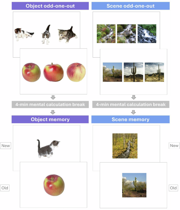
Forty-eight triplets of object pictures and 48 triplets of scene pictures were selected from existing databases (objects^{74,75,76,77,78,79,80}; scenes^81,82,83). In each triplet, two pictures represented the same object or the same scene, but from different viewpoints, and the third picture represented another exemplar of the same concept of object or scene.

Recognition memory

We selected one picture from each of the 48 triplets of the previous phase for each condition, object or scene (16 of them were the targets, viewpoint 1, 16 were the targets, viewpoint 2, and 16 were the ‘odd’ ones). We then matched each of these pictures with a new picture, i.e. the lure, representing another exemplar of the same concept. This resulted in 48 new object pictures and 48 new scene pictures. This task and the odd-one-out task are illustrated in Fig.1.

Visual similarity measures

We assessed the complex visual properties of our image sets by evaluating the similarity of visual features derived from the pre-trained CNN AlexNet. AlexNet was trained on 1.2 million high-resolution images, categorising them into 1000 distinct categories (or classes). AlexNet consists of eight layers, including five convolutional layers (conv1 – conv5) and three fully connected layers (fc6 – fc8). Each convolutional layer takes input from the previous layer, using filters sensitive to different types of visual input⁸⁴. By construction, the filters of the first convolutional layers capture low-level properties of stimuli, such as edges with specific spatial frequencies and orientations, as well as colour information⁸⁵while the later layers detect more complex visual features, such as the presence of specific visual objects or object parts (e.g. dog legs, bird eyes), across various spatial scale and viewing angles⁸⁵. To obtain the activation values from the CNN for our set of images, we presented each image (objects and scenes separately) to the pre-trained network, which generated activation values for each node in each layer for each image.

To reduce the number of measures analysed and because consecutive layers are highly correlated, we extracted the activation values for three representative layers for each image (layers conv3, fc6 and fc7, corresponding to early, middle, and late layers, respectively). For each of these layers, we compared the activation values of each image against all other images in the dataset (objects and scenes separately, N = 192 images per set) using Euclidian distance, producing a similarity matrix for each layer.

For the odd-one-out task, we extracted the Euclidean distance between the value of the ‘odd’ image in each triplet and its two associated target images for each representative layer. The average of these two distances was used to compute a single value of visual distance per triplet. For the recognition memory task, we extracted the Euclidean distance between the target image and its corresponding lure.

Here, we present data analysed using the late visual layer (fc7); information and analyses on other layers (conv3 and fc6), as well as from human subjective ratings of visual distance acquired through a pilot study, can be found in the Supplementary Methodsand Supplementary Results.

Procedure

Data collection took place at the research centre, in a dedicated testing room. The experimenter explained task instructions and then left the room during the completion of the tasks by the participants, who did so on a laptop. The experimenter remained available in the next room to answer questions, if any. This study was part of a longer protocol that included other tasks, so participants had to come twice to the lab. For this study, the total acquisition duration was of about 2 h.

Odd-one-out task

Object and scene tasks were built using PsychoPy⁸⁶. For each trial, the three pictures of a triplet were presented side by side on the screen. The order of trials was randomised across participants. Participants were instructed to identify the item that represented a different exemplar than the other two items, using the left, down and right arrow keys, depending on the item’s position on the screen (left-side, middle, or right-side of the screen, respectively). Each trial ended with the participant’s keypress or, in the absence of such, lasted a maximum of 10 s. An absence of response was treated as an incorrect response. This was followed by a 500 ms blank screen and a 500 ms fixation cross before the start of the next trial. Conditions for scenes and objects were presented in separate blocks. The subsequent memory test started only after the entire odd-one-out block (objects or scenes) was completed. Once the memory test for one condition was finished, participants proceeded to the odd-one-out task for the other condition, followed by its respective memory test. The order of object and scene conditions was counterbalanced across participants. The task is illustrated in Fig.1.

Recognition memory

There was a 4-min break between the odd-one-out task and the start of the memory task (object or scene), filled with calculations. For the memory test, items were presented one by one on the screen (48 targets and 48 lures) in a pseudo-randomised order. Participants were instructed to determine, for each item, whether it had been seen in the previous task or not, answering with the « a » and « p » keys. Each trial ended with participants’ keypress, or in the absence of such, lasted a maximum of 6 s, and was followed by a 500 ms blank screen and a 500 ms fixation cross, before the start of the next trial.

MRI acquisitions

Images were acquired on a 3 T Siemens Prisma scanner with a 64-channel head coil. Two anatomical images were acquired: a T1-weighted structural MRI (acquisition matrix = 256 × 240 × 224, voxel size = 1 × 1 × 1 mm³) and a high-resolution T2-weighted structural MRI (acquisition matrix = 448 × 448 × 60, voxel size = 0.4 × 0.4 × 1.2 mm³) with a partial field of view covering the entire MTL with an oblique coronal orientation perpendicular to the long axis of the hippocampus. The quality of each image was systematically visually checked, especially the T2-MRI, which is highly sensitive to motion (after reminding the participant to stay still during the entire subsequent 8 min of acquisition), and re-run in case of poor quality due to excessive motion. When T2 images were acquired twice (N = 7), we selected the one with the best quality for further processing. In addition, multislice T2*-weighted, eyes open, resting-state functional images were acquired with the multi-band gradient-echo echo-planar imaging sequence (CMRR, University of Minnesota) using axial slice orientation and covering the whole brain (36 slices, multiband factor = 2, FoV =  216 × 216 mm²voxel size 3 × 3 × 3 mm³25% interslice gap, matrix size 72 × 72 × 36, TR = 1.7 s, TE = 30 ms, FA = 90°). The three initial volumes were discarded to avoid T1 saturation effects.

Data preprocessing

All data were BIDsified using an automated pipeline⁸⁷.

MTL regions segmentation

High-resolution T2-weighted MRI images were labelled using the Automatic Segmentation of Hippocampal Subfields software package (with atlas package ‘ashs_atlas_upennpmc_20161128’ obtained from the NITRC repository made available on the ASHS website)⁵⁸. The hippocampal subfields, the ErC, BA35 and BA36 in the left and right hemispheres were thereby labelled in each participant. Each output from ASHS underwent visual quality control.

The ErC was further manually subdivided into alErC and pmErC, following established protocols from previous studies (e.g. refs. 25,52). Intra-rater reliability was assessed by separately comparing the segmentation of the right and left alErC of five randomly selected scans, completed by the same rater (ED) after a delay of 6–8 months. Consistency between measurements was evaluated using intraclass ICC using the type (3, B) to compute intra-rater consistency⁸⁸ and spatial overlap was assessed with the Dice metric (using the mean Dice value across the selected scans; Dice values are derived using the formula 2*[intersecting volume]/[original segmentation volume + repeat segmentation volume]). Both measures fall between 0 and 1, with higher values indicating greater reliability. Figure2 illustrates the results of the segmentation, both automated and manual, for the al- and pm-ErC of the MTL.

For all subregions belonging to ErC and perirhinal cortex (BA35 and BA36), volumes were normalised by the extent of their segmentation in the slice direction (hippocampal axis), by dividing their volume by the product of the number of slices and the slice thickness⁵⁸. Additionally, all regional volumes were adjusted before analyses to account for total estimated intracranial volume (ICV) for each participant using the formula Volume_adjusted = Volume_raw − β_ICV(ICV_indiv – ICV_mean), where β refers to the regression coefficient of the model on a given regional volume of interest while using ICV as a predictor. This approach is based on extensive prior work (e.g. refs. ^26,27,30).

The volume of our main region of interest, the tErC, was then computed as the sum of BA35 and alErC.

ROI definition

These MTL regions were additionally used as seeds and ROIs for resting-state connectivity analyses. To do so, left and right hemispheres atlases were coregistered to the subject’s T1 space using the transformation matrix provided by ASHS and the flirt function of FSL⁸⁹. Similar to the volumetric analyses, BA35 and alErC regions were merged into one single tErC label using FSL.

To ensure that all ROIs had reliable signal despite the susceptibility artefact causing signal dropout in the MTL⁶⁸we calculated the mean signal across the total grey matter and excluded voxels with signal < 25% of the mean grey matter signal for each participant³⁹.

In addition to the MTL ROIs (i.e. left and right CA1, CA3, pmErC, BA36, tErC and PhC), we also identified a set of predefined ROIs for the ROI-to-ROI analysis, based on the existing literature, which have shown strong connectivity with the MTL and belong to the PM-AT network. Specifically, within the AT system, these include the left and right superior frontal gyrus, orbito-frontal cortex, temporal pole, and medial prefrontal cortex. As part of the PM system, we included the left and right angular gyrus, superior and inferior lateral occipital cortex, precuneus, thalamus, and PCC (see in ref. ¹⁵). The ROIs were defined using the atlas provided by the CONN toolbox. Of note, the results from this analysis were similar when replicating the analysis using predefined ROIs from the atlas used by Berron et al.¹⁵so here we only present analyses on ROIs extracted from the CONN atlas.

Functional MRI data preprocessing

MRI data preprocessing was conducted with SPM 12 (Wellcome Trust Center for Neuroimaging, London, UK). For each subject, EPI time series were corrected for motion and distortion using Realign and Unwarp⁹⁰and coregistered to the corresponding structural image. The structural image was then segmented into grey and white matter using the ‘unified segmentation’ approach⁹¹. The warping parameters were subsequently applied separately to the functional and structural images to produce normalised images with isotropic voxel size of 2 mm for functional images and 1 mm for structural images. No spatial smoothing was performed to preserve the high resolution of the images and enable more accurate signal quantification within spatially adjacent subregions. Potential outlier scans were identified using ART⁹² as acquisitions with framewise displacement above 0.9 mm or global BOLD signal changes exceeding five standard deviations^93,94. A reference BOLD image was computed for each subject by averaging all scans, excluding outliers.

Denoising and further analyses were conducted using CONN toolbox, release 22.a^95,96. Functional data were denoised using a standard pipeline, which involved regressing potential confounding effects including white matter timeseries (5 CompCor noise components), CSF timeseries (5 CompCor noise components), movements regressors (6 components), outlier scans (below 252 factors)⁹⁴session effects and their first order derivatives (2 factors), and linear trends (2 factors) within each functional run. This was followed by bandpass frequency filtering of the BOLD timeseries⁹⁷ between 0.008 Hz and 0.09 Hz. CompCor^98,99 noise components within white matter and CSF were estimated by computing the average BOLD signal as well as the largest principal components orthogonal to the BOLD average, and outlier scans within each subject’s eroded segmentation masks. Considering the number of noise terms included in this denoising strategy, the effective degrees of freedom of the BOLD signal after denoising were estimated to range from 47 to 95.4 (average 92.6) across all subjects.

Statistical analyses

Behavioural analyses

Behavioural analyses were run on JASP¹⁰⁰ for t-tests comparisons (1) to chance level (i.e. 0; one-sided one sample t-tests) and (2) between objects and scenes conditions in the memory task (i.e. two-sided paired sample t-tests), as well as on RStudio version 2023.12.1¹⁰¹ for Generalised Linear Mixed Models (GLMM; see below) on a trial-by-trial basis to account for the accuracy binary outcome (0, 1) of the dependent variables. GLMMs were fit with the package lme4¹⁰². GLMMs were run in each task separately (odd-one-out and recognition memory), with condition (object or scene) as within-subject factor, visual distance computed from the highest layer of AlexNet (fc7) as continuous predictor, applying a centre-scale (i.e. the mean of the variable was subtracted from each data point, shifting the mean to 0), and participant’s ID as random factor. Following these GLMMs, post-hoc pairwise comparisons were carried out on estimated marginal means for a given effect of interest, with Tukey’s adjustments when there were multiplicity issues using the emmeans package¹⁰³ and the function lstrends from lsmeans package to deal with continuous factors. Estimated marginal means from the models are reported.

In the odd-one-out task, the dependent variable was accuracy on each discrimination trial. In the GLMMs for the recognition memory task, because we were interested in discrimination abilities with increasing visual distance between the target and its matched lure, behavioural analyses were run on accuracy for lures (i.e. correct rejections of lures as a function of their visual distance with the target). While each target and its matched lure were presented during the yes-no recognition task, we decided to focus this analysis on the lures that were presented before the target, to avoid effects of target repetition on subsequent lure discrimination. We additionally compared the mean correct recognition (hit) rates and discrimination indices (Hits minus False Alarms) between objects and scenes using paired sample t-tests (therefore, not including visual distance, as a target cannot be visually distant from itself).

Plots of the results were generated using the ggplot2 package¹⁰⁴.

Volumes regression analyses

To explore the relationship between MTL structures integrity and the impact of visual distance on performance, we computed measures of « accuracy sensitivity to visual similarity » for each subject, by relating accuracy in each trial with the trial’s index of visual distance using Pearson correlations, and then transforming each r-value obtained for each participant by a Fisher transformation to give a Z-score. These correlations were computed separately for objects and scenes, and separately for each task (accuracy in the odd-one-out task, and lures discrimination accuracy in the recognition memory task). The participant’s resulting « sensitivity to visual similarity » indices were then related to MTL structures integrity (volumes) using linear regressions with the forward stepwise method (allowing to avoid issues of multicollinearity between measures) in JASP¹⁰⁰with 12 ROIs: left and right CA1, CA3, pmErC, BA36, tErC and PhC. See in refs. ^32,30 for similar methods.

The same analyses, but using human subjective ratings of similarity, and layers 3 and 6 of AlexNet are presented in Supplementary Results.

Resting-state functional connectivity analyses

Seed-based connectivity

Seed-based connectivity maps were estimated, characterising the spatial pattern of functional connectivity with a seed area while controlling for all other seeds. Seed regions included the 12 ROIs from the MTL. Functional connectivity strength was represented by Fisher-transformed semi-partial ICC (thus allowing controlling for any signal bleed between adjacent regions) from a weighted general linear model (GLM), estimated separately for each target voxel, modelling the association between all seeds simultaneously and each individual voxel BOLD signal timeseries. To compensate for possible transient magnetisation effects at the beginning of each run, individual scans were weighted by a step function convolved with an SPM canonical hemodynamic response function and rectified.

Then, group-level analyses were performed using a GLM. For each individual voxel, a separate GLM was estimated, with first-level connectivity measures at this voxel as dependent variables and participant’s ID as independent variable. Voxel-level hypotheses were evaluated using multivariate parametric statistics with random-effects across subjects and sample covariance estimation across multiple measurements. Inferences were performed at the level of individual clusters (groups of contiguous voxels). Cluster-level inferences were based on parametric statistics from Gaussian Random Field theory¹⁰⁵. Results were thresholded using a combination of a cluster-forming p < 0.001 voxel-level threshold, and a familywise corrected p FDR < 0.05 cluster-size threshold¹⁰⁶. Subsequently, contrasts were run between the first-level connectivity measures associated with sensitivity to visual similarity indices in the objects versus scenes conditions, separately for the odd-one-out and the recognition memory task.

ROI-to-ROI functional connectivity

In the first-level analysis, ROI-to-ROI connectivity matrices were estimated for each participant to characterise the functional connectivity between each pair of regions, including the 12 ROIs from the MTL, as well as additional ROIs belonging to the PM-AT systems (29 ROIs in total, see Fig.5). Functional connectivity strength was represented by Fisher-transformed semi-partial correlations, which allowed controlling for any signal bleed between adjacent regions. Coefficients from a weighted-GLM were estimated separately for each pair of ROIs, which characterised the association between their BOLD signal time series. To compensate for possible transient magnetisation effects at the beginning of each run, individual scans were weighted by a step function convolved with an SPM canonical hemodynamic response function and rectified.

Then, at the group level, a first analysis was performed in CONN using a GLM to characterise the pattern of functional connectivity among all the ROIs. For each individual connection, a separate GLM was estimated, with first-level connectivity measures at this connection as dependent variables and participant’s ID as independent variable. Connection-level hypotheses were evaluated using multivariate parametric statistics with random effects across subjects and sample covariance estimation across multiple measurements. Inferences were performed at the level of individual clusters (groups of similar connections). Cluster-level inferences were based on parametric statistics within- and between- each pair of networks¹⁰⁷with networks identified using a complete-linkage hierarchical clustering procedure based on ROI-to-ROI anatomical proximity and functional similarity metrics. Results were thresholded using a combination of a p < 0.05 connection-level threshold and a familywise corrected p FDR < 0.05 cluster-level threshold.

Then, first-level connectivity strength values for each connection and each subject were extracted to perform linear regression analyses with the forward stepwise method, to assess the association between the connections among selected ROIs and the indices of sensitivity to visual similarity, tested one at a time (4 indices in total, derived from object and scene conditions, for both odd-one-out and recognition memory tasks). These analyses were run in JASP¹⁰⁰. To reduce the number of measures entered in the analysis, we ran separate analyses including exclusively regions from the AT system and the hippocampus on one hand (i.e. AT system: bilateral tErC, BA36, superior frontal gyrus, orbito-frontal cortex, temporal pole, and medial prefrontal cortex; hippocampus: bilateral CA1 and CA3), and of the PM system and the hippocampus on the other hand (i.e. bilateral pmErC, PhC, angular gyrus, superior and inferior lateral occipital cortex, precuneus, thalamus, and PCC). Additionally, we restricted the analyses to selected hypotheses-driven connections involving tErC connectivity and pmErC connectivity, respectively.

Reporting summary

Further information on research design is available in theNature Portfolio Reporting Summary linked to this article.